Part 1: Fit a Neural Field to a 2D Image
For fitting a Neural Field to a 2D Image, we are using \(F: \{u, v\}\rightarrow \{r, g, b\}\).
in which \(\{u, v\}\) is the pixel coordinate. The network is an Multilayer Perceptron (MLP) network with Sinusoidal
Positional Encoding (PE) that takes in the 2-dim pixel coordinates, and output the 3-dim pixel colors. PE is
is an operation that applies a serious of sinusoidal functions to the input cooridnates, to expand its dimensionality:
\[PE(x) = \{x, sin(2^0\pi x), cos(2^0\pi x),
sin(2^1\pi x), cos(2^1\pi x), ..., sin(2^{L-1}\pi x), cos(2^{L-1}\pi x)\}\] in which \(L\) is the highest frequency level. You can
start from \(L=10\) that maps a 2 dimension coordinate to a 42 dimension vector.
We are using a dataloader that randomly samples \(N\) pixels at every
iteration for training, which returns both the \(N\times2\) 2D coordinates and \(N\times3\) colors of the
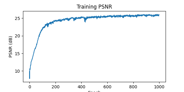
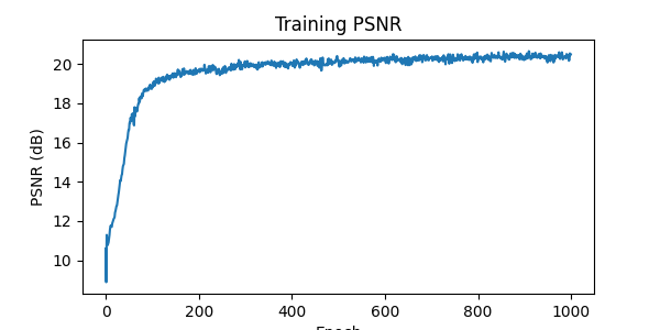
pixels. The model is trained with using Adam (torch.optim.Adam) with a learning rate of 1e-2 and mean squared error loss (MSE) (torch.nn.MSELoss).
The metric is using PSNR from MSE: \[PSNR = 10 \cdot log_{10}\left(\frac{1}{MSE}\right)\].
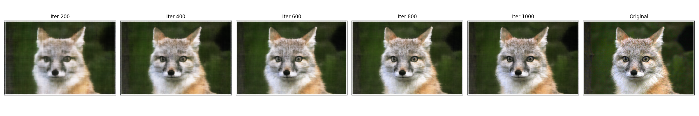
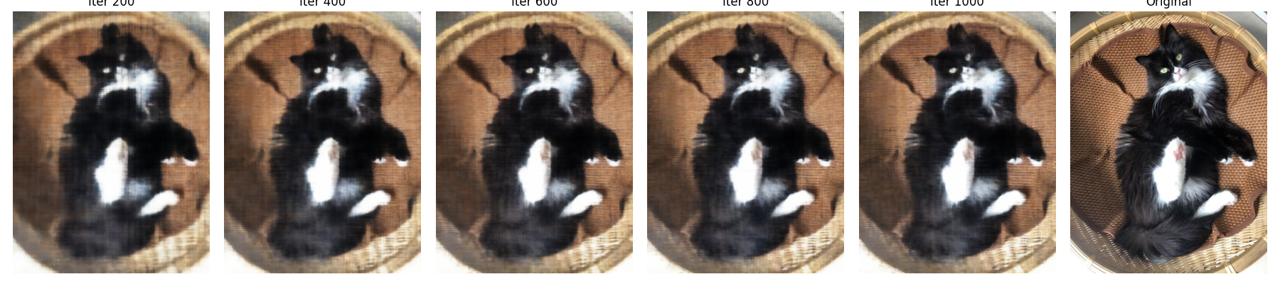
After 1000 iterations, the training PSNR and predicted images every 200 iterations are illustrated below:
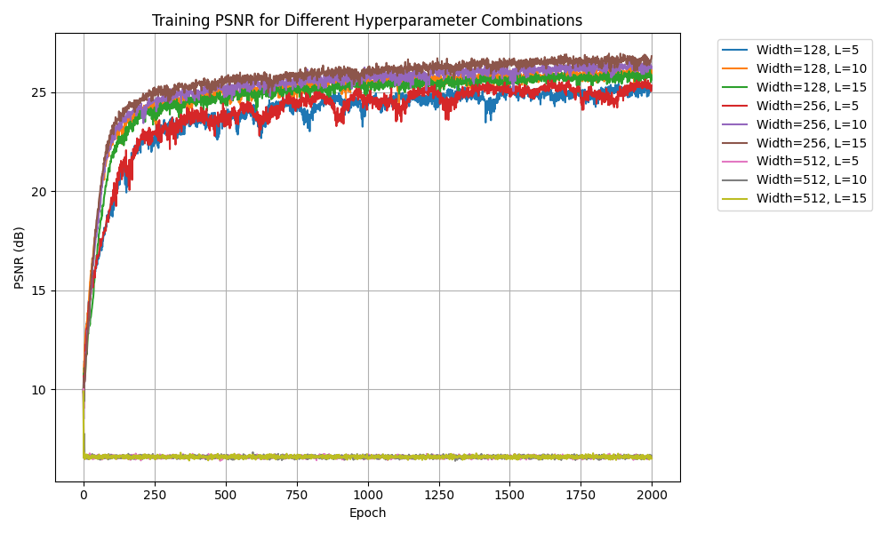
Hyperparameter Tuning: Varying two of the hyperparameters, the channel size and max frequency, the resulted PSNRs are recorded:
from the graph, it can be concluded that increasing channel size from 128 to 256 can improve the model performance, and increasing the max frequency
can also increase the model performance. However, when the channel size is 512, the PSNR drops significantly. This is probably due to
vanishing gradients and too many parameters for the large channel size model.
Part 2: Fit a Neural Radiance Field from Multi-view Images
To represent 3D space, Neural Radiance Field uses \(F: \{x, y, z, \theta, \phi\} \rightarrow \{r, g, b,
\sigma\}\), through inverse rendering from multi-view calibrated images.
We are using the Lego scene from the original NeRF paper, with lower resolution images (200 x 200) and preprocessed cameras.
Create Rays from Cameras
Camera to World Coordinate Conversion:
The transformation between the world space \(\mathbf{X_w} = (x_w, y_w, z_w)\) and the
camera space \(\mathbf{X_c} = (x_c, y_c, z_c)\) is defined as a rotation matrix \(\mathbf{R}_{3\times3}\) and a translation vector
\(\mathbf{t}\):
\[\begin{align} \begin{bmatrix} x_w \\ y_w \\ z_w \\ 1 \end{bmatrix}
= \begin{bmatrix} \mathbf{R}_{3\times3} &
\mathbf{t} \\ \mathbf{0}_{1\times3} & 1 \end{bmatrix}^{-1} \begin{bmatrix} x_c \\ y_c \\ z_c \\ 1 \end{bmatrix} \end{align}\]
in which
\(\begin{bmatrix} \mathbf{R}_{3\times3} & \mathbf{t} \\ \mathbf{0}_{1\times3} & 1 \end{bmatrix}\) is the world-to-camera
(w2c) matrix. From the camera-to-world transformation matrix and camera coordinates, we
implement x_w = transform(c2w, x_c).
Pixel to Camera Coordinate Conversion:
For a pinhole camera with focal length \((f_x, f_y)\) and principal point \((o_x =
\text{image_width} / 2, o_y = \text{image_height} / 2)\), it's intrinsic matrix \(\mathbf{K}\) is defined as: \[\begin{align}
\mathbf{K} = \begin{bmatrix} f_x & 0 & o_x \\ 0 & f_y & o_y \\ 0 & 0 & 1 \end{bmatrix} \end{align}\] which can be used to project a 3D
point \((x_c, y_c, z_c)\) in the camera coordinate system to a 2D location \((u, v)\) in pixel coordinate system :
\[\begin{align} \begin{bmatrix} x_c \\ y_c \\ z_c \end{bmatrix} = \mathbf{K}^{-1} s \begin{bmatrix} u \\ v \\ 1 \end{bmatrix} \end{align}\]
in which \(s=z_c\) is the depth of this point along the optical axis. To implement it, we define
x_c = pixel_to_camera(K, uv, s).
Pixel to Ray:
A ray can be defined by an origin \(\mathbf{r}_o \in R^3\) vector and a direction \(\mathbf{r}_d \in R^3\)
vector. We want to know the \(\{\mathbf{r}_o, \mathbf{r}_d\}\) for every pixel \((u, v)\). The
origin \(\mathbf{r}_o\) of those rays is the location of the cameras: \[\begin{align} \mathbf{r}_o =
-\mathbf{R}_{3\times3}^{-1}\mathbf{t} \end{align}\] The ray direction for pixel \((u, v)\) is computed by choosing a point
along this ray with depth equals 1 (\(s=1\)) and find its coordinate in the world space \(\mathbf{X_w}\). Then the
normalized ray direction can be computed by: \[\begin{align} \mathbf{r}_d = \frac{\mathbf{X_w} - \mathbf{r}_o}{||\mathbf{X_w} -
\mathbf{r}_o||_2} \end{align}\] To convert a pixel coordinate to a ray with origin and
noramlized direction: ray_o, ray_d = pixel_to_ray(K, c2w, uv), from x_c = pixel_to_camera(K, uv, s), x_w = transform(c2w, x_c).
Sampling
At every training iteration, we flatten all pixels from all images and do a global sampling once to get N rays from all images. Then discritize each ray into samples that live in the 3D space
by uniformly creating samples along the ray (t = np.linspace(near, far, n_samples)), with near=2.0, far=6.0, n_samples=64.
The actually 3D corrdinates can be accquired by \(\mathbf{x} = \mathbf{R}_o + \mathbf{R}_d * t\), and introduce small perturbation 0.2 during training.
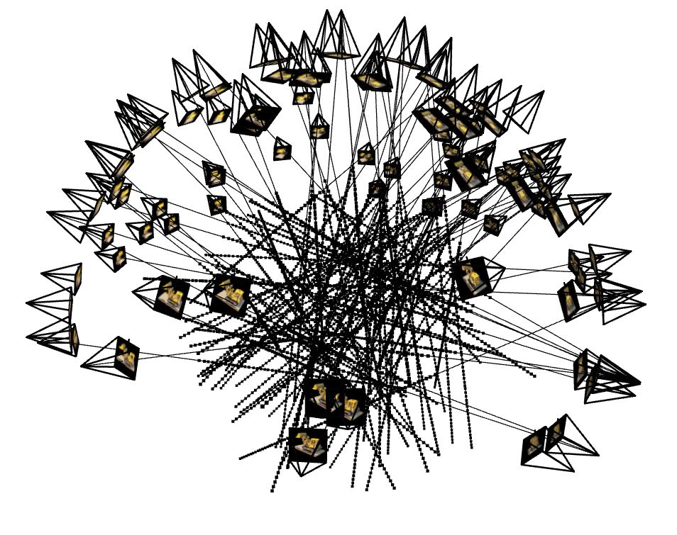
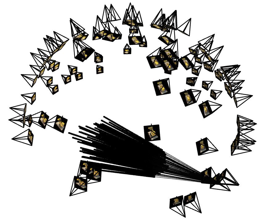
Visualization of cameras, rays, and samples in 3D
This first visualization shows all training cameras, with 100 randomly sampled rays in the scene. The second visualization shows 100 rays sampled from the first image. They are captures produced using the code from the project website.
Neural Radiance Field Network
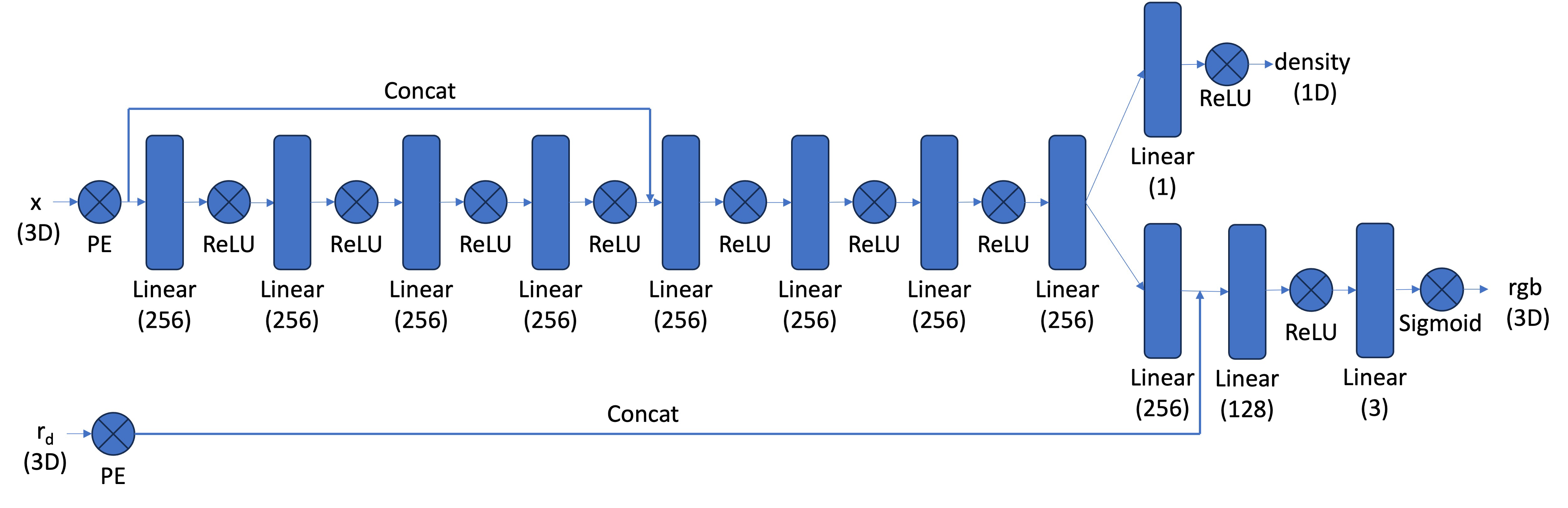
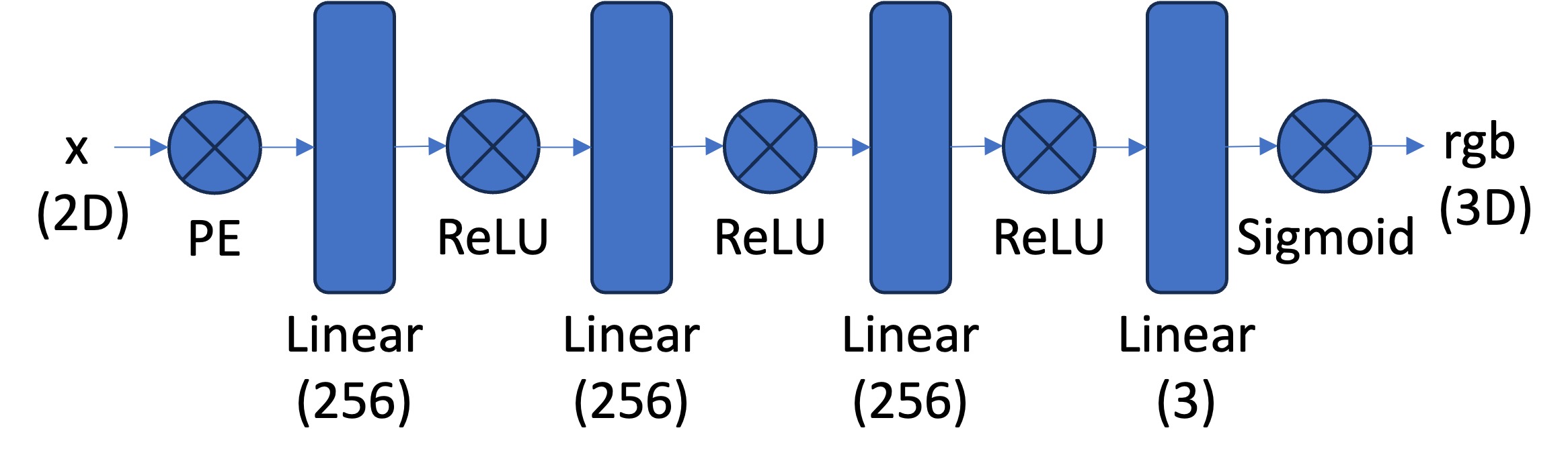
The network is a MLP that takes 3D world coordinates, 3D vector ray direction as input. It would predicted the the color and density for the 3D points.
The world coordinates is encoded by PE with L=10, while the ray direction is encoded with L=4. The network architecture follows the structure shown in the graph, with several modifications. Residual blocks have been added at three locations: before and after concatenating the world coordinates, and after concatenating the world coordinates with ray directions.
Volume Rendering
The core volume rendering equation is as follows: \begin{align} C(\mathbf{r})=\int_{t_n}^{t_f} T(t) \sigma(\mathbf{r}(t))
\mathbf{c}(\mathbf{r}(t), \mathbf{d}) d t, \text { where } T(t)=\exp \left(-\int_{t_n}^t \sigma(\mathbf{r}(s)) d s\right)
\end{align}
The discrete approximation (thus tractable to compute) of this equation can be stated as the following: \begin{align}
\hat{C}(\mathbf{r})=\sum_{i=1}^N T_i\left(1-\exp \left(-\sigma_i \delta_i\right)\right) \mathbf{c}i, \text { where } T_i=\exp
\left(-\sum{j=1}^{i-1} \sigma_j \delta_j\right) \end{align}
where \(\textbf{c}_i\) is the color obtained from our network at sample location \(i\), \(T_i\) is the probability of a ray not terminating before sample location \(i\), and \(1 - e^{-\sigma_i \delta_i}\) is the probability of terminating at sample location \(i\). This discrete approximation is implemented in the volrend function, which computes the weights using the weights function and performs the weighted sum to obtain the final color. The sampling points along rays where we evaluate these quantities are generated using the sample_along_rays function.
After the model returns the densities and colors, we use the discrete approximation above to render the final pixel color in the resulting image.
Bells & Whistles: coarse-to-fine PDF resampling
To improve sampling efficiency, we implement a hierarchical sampling strategy that concentrates samples where they most affect the final rendering. This is achieved using two networks - a coarse and a fine network - that are optimized simultaneously.
First, using sample_along_rays, we sample Nc=64 locations through stratified sampling and evaluate the coarse network. The render_rays function processes these points through the coarse network to obtain initial densities and colors.
Then, to focus sampling on the most relevant parts of the volume, we use the coarse network's output to guide a second, more informed sampling. This is done by rewriting the alpha composited color from the coarse network as \(\hat{C_c}(r) = \sum^{N_c}_{i=1} w_ic_i), w_i = T_i\left(1-\exp \left(-\sigma_i \delta_i\right)\right )\). These weights are computed by our weights function.
The weights are normalized to create a piecewise-constant PDF along the ray. Using sample_pdf, we perform inverse transform sampling to generate Nf=128 additional samples from this distribution. The fine network then evaluates both the original coarse samples and these new samples (Nc+Nf total), and the final color is rendered using the volrend function with all samples.
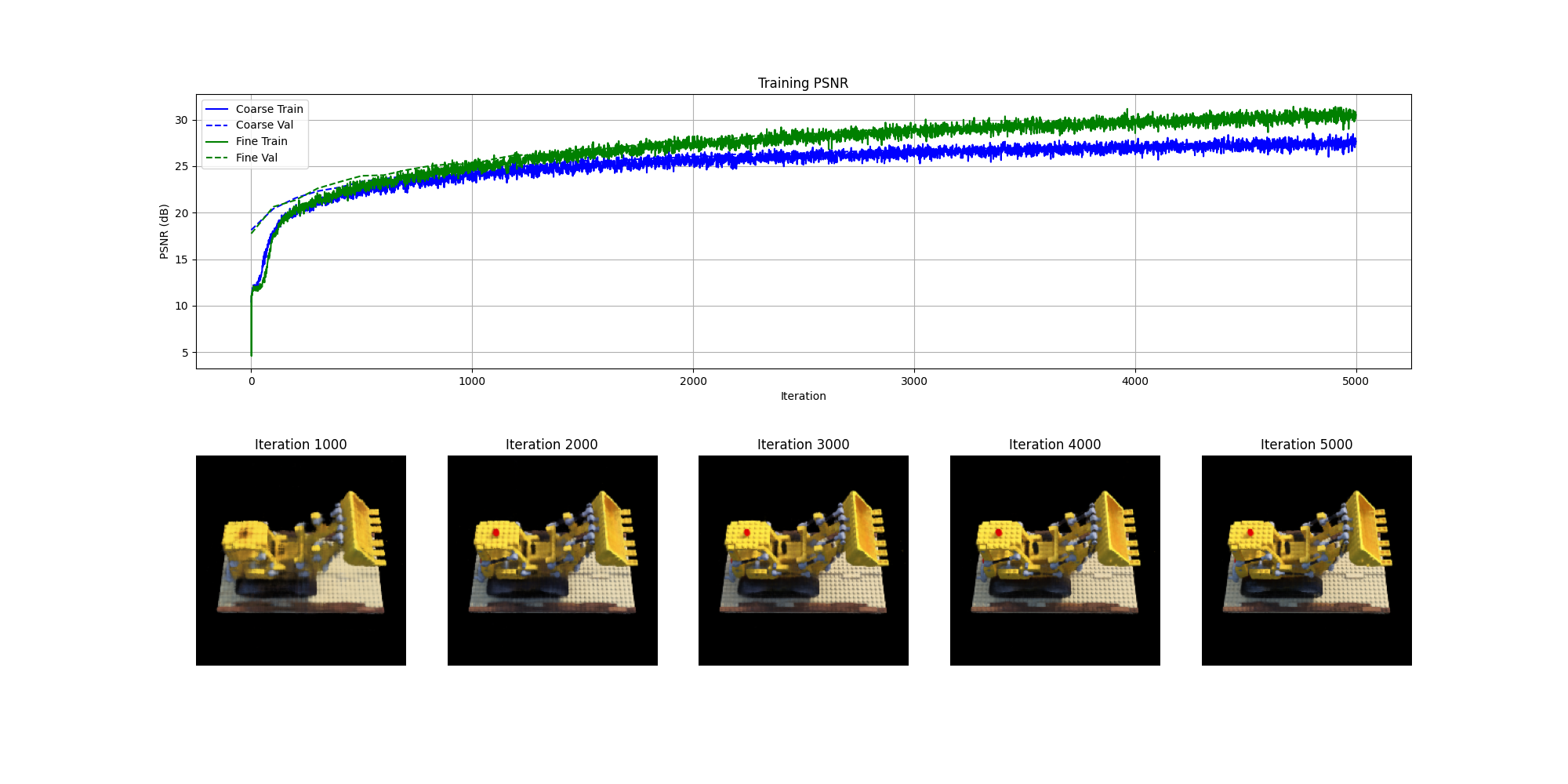
Result
The model is trained using the Adam optimizer (torch.optim.Adam) with a learning rate decaying from 1e-3 to 1e-4, and the mean squared error (MSE) loss (torch.nn.MSELoss).
Performance is evaluated using the Peak Signal-to-Noise Ratio (PSNR) metric, calculated from the MSE values. Each training iteration processes a batch of 2500 randomly sampled rays. The model is trained for 5000 iterations, and a spherical rendering of the lego video using the provided cameras extrinsics
are displayed below:
Bells & Whistles: Improve PSNR to 30+
By adding additional residual blocks, and increase the training time to 5000 iterations, the PSNR of the fine network reaches 30+ db.
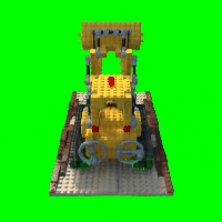
Bells & Whistles: Render the Lego video with a different background color
To incorporate a background color into the rendering, we first calculate the probability that light travels through the entire volume without being scattered or absorbed. We then blend the accumulated rendering with the background color, weighting the background contribution by this probability to ensure that areas with high transmittance display the background appropriately.