CS180 Project #5: Fun With Diffusion Models
Part A: The Power of Diffusion Models
In the following section, a pretrained DeepFloyd denoisers with \(T=1000\) is used to produce high quality images as the description.
Part 0: Setup
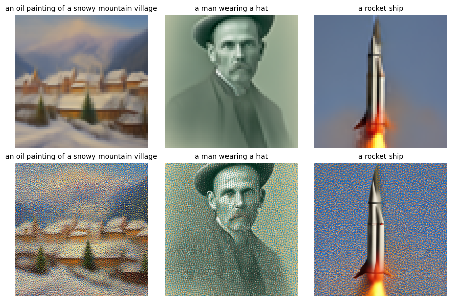
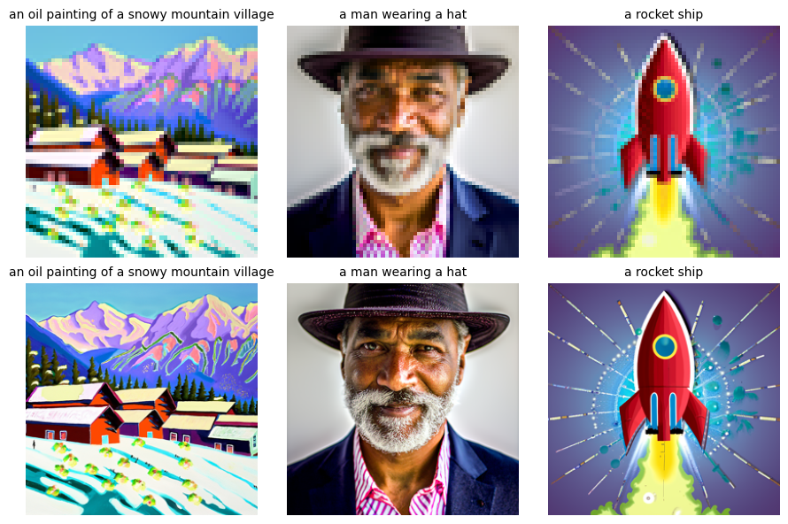
For the 3 text prompts, the caption and the output of the model for num_inference_steps=5, 100 with seed=0 are displayed below:


It can be seen that the model generate images resembling the text prompts, and as the num_inference_steps
increases, the images have higher quality and more details. And after passed into stage_2, the quality improves.
Part 1: Sampling Loops: 1.1 Implementing the Forward Process
The forward process takes a clean image and adds noise to it. It is defined by: $$q(x_t | x_0) = N(x_t ; \sqrt{\bar\alpha} x_0, (1 -
\bar\alpha_t)\mathbf{I})$$ which is equivalent to computing
$$ x_t = \sqrt{\bar\alpha_t} x_0 + \sqrt{1 - \bar\alpha_t} \epsilon
\quad \text{where}~ \epsilon \sim N(0, 1) $$
That is, given a clean image \(x_0\), we get a noisy image \(x_t\) at
timestep \(t\) by sampling from a Gaussian with mean \(\sqrt{\bar\alpha_t}x_0 \) and variance \( (1 - \bar\alpha_t) \).
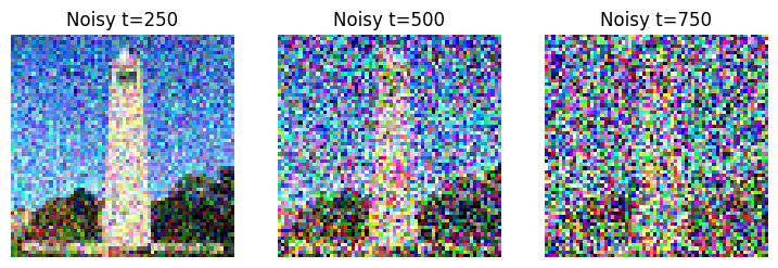
The test images at noise level [250, 500, 750] are shown below:

1.2 Classical Denoising
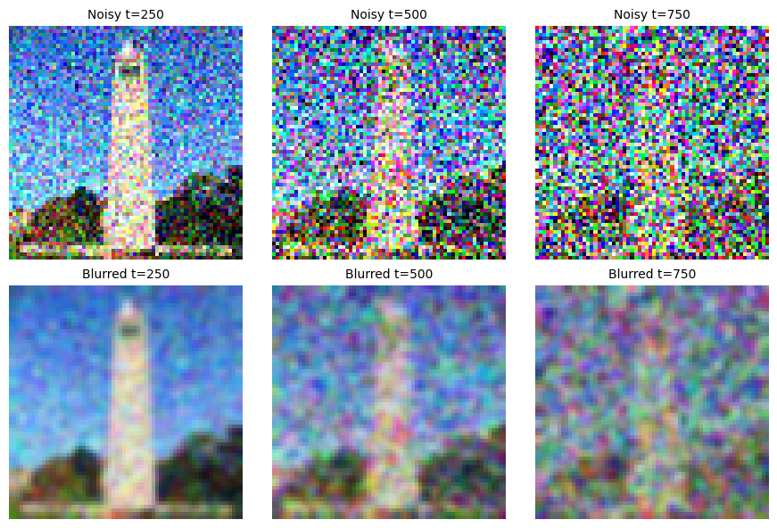
Take noisy images for timesteps [250, 500, 750], and use
torchvision.transforms.functional.gaussian_blur to remove the noise.
The test images using kernel_size=(5, 5), sigma=(1, 1) are shown below:

1.3 One-Step Denoising
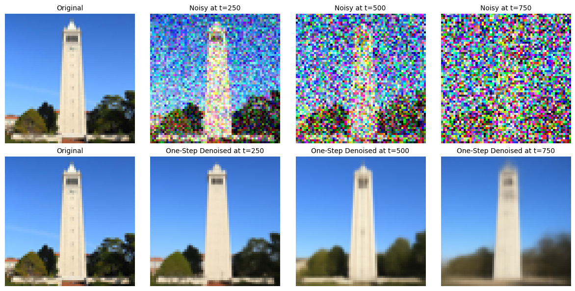
In this section, a pretrained diffusion model is used to recover Gaussian noise from the image,
Then, we can remove this noise to recover the original image.
Because this diffusion model was trained with text conditioning, a text prompt embedding for the prompt "a high quality photo" is applied.
The original image, the noisy image, and the estimate of the original image are shown below:

1.4 Iterative Denoising
In this section, the diffusion model is used to denoise iteratively for \(T=1000\).
The process is sped up by skipping steps by creating a new list of timesteps.
On the ith denoising step, apply the following formula for update:
$$ x_{t'} = \frac{\sqrt{\bar\alpha_{t'}}\beta_t}{1 - \bar\alpha_t} x_0 +
\frac{\sqrt{\alpha_t}(1 - \bar\alpha_{t'})}{1 - \bar\alpha_t} x_t +
v_\sigma$$
where:
- \(x_t\) is the image at timestep \(t\)
- \(x_{t'}\) is the noisy image at timestep \(t'\) where \(t' < t\)
- \(\bar\alpha_t\) is defined by
alphas_cumprod
- \(\alpha_t = \frac{\bar\alpha_t}{\bar\alpha_{t'}}\)
- \(\beta_t = 1 - \alpha_t\)
- \(x_0\) is the current estimate of the clean image
The noisy image every 5th loop of denoising, the final predicted clean image using iterative denoising with previous denoised images are shown below:


1.5 Diffusion Model Sampling
By setting i_start = 0 and passing in random noise, images can be generated from scratch.
5 sampled images are shown below:

1.6 Classifier-Free Guidance (CFG)
By using a technique called Classifier-Free Guidance, the image quality can be greatly improved.
In CFG, both a conditional and an unconditional noise estimate are computed, denoted as
\( \epsilon_c \) and \( \epsilon_u \).
Then, the new noise estimate be: $$\epsilon = \epsilon_u + \gamma
(\epsilon_c - \epsilon_u) $$
where \( \gamma \) controls the strength of CFG.
When \( \gamma > 1 \), the image quality can be much higher.
5 images of "a high quality photo" with a CFG scale of \( \gamma > 7 \) are shown below:

1.7 Image-to-image Translation
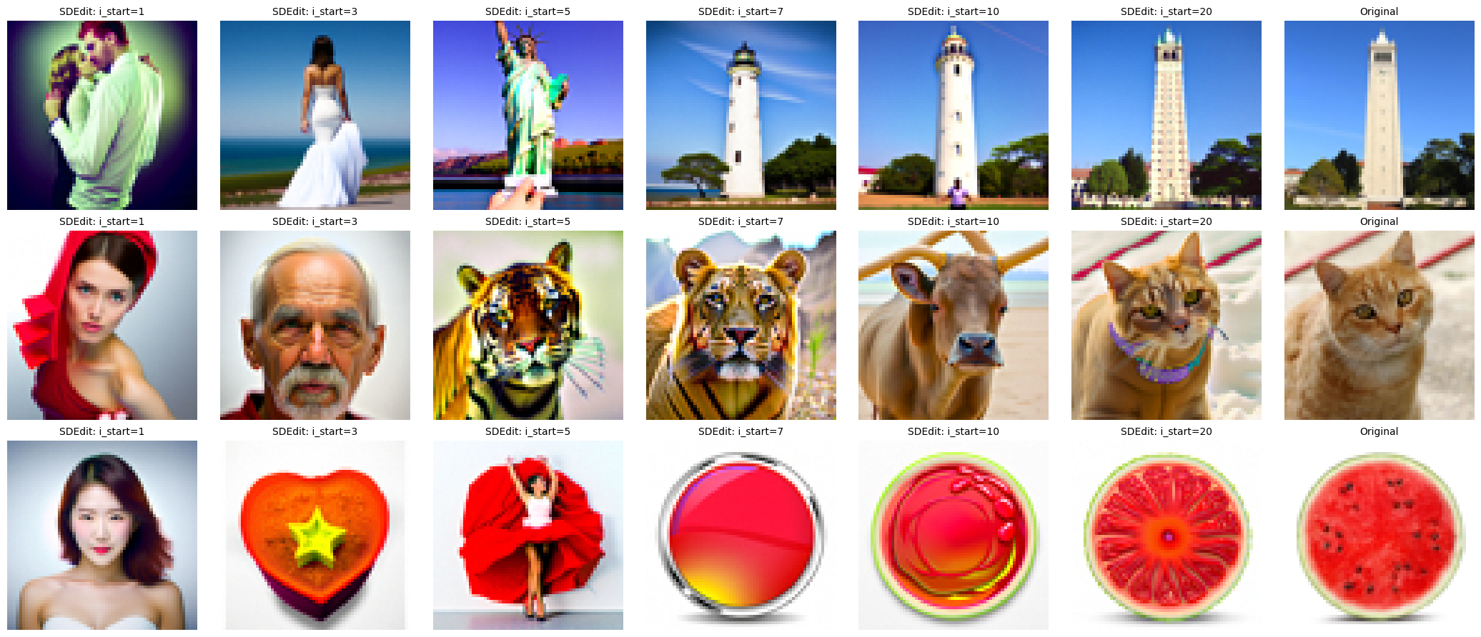
The SDEdit algorithm is used such that the original test image is noised a little, and be forced back onto the image manifold without any conditioning
to create an image that is similar to the test image.
Edits of the test images, using the given prompt at noise levels [1, 3, 5, 7, 10, 20] with text prompt "a high quality photo" are shown below:

1.7.1 Editing Hand-Drawn and Web Images
This procedure works particularly well if starting with a nonrealistic image and project it onto the natural image manifold.
For noise levels [1, 3, 5, 7, 10, 20], 1 image from the web and 2 hand drawn images are shown below.


1.7.2 Inpainting
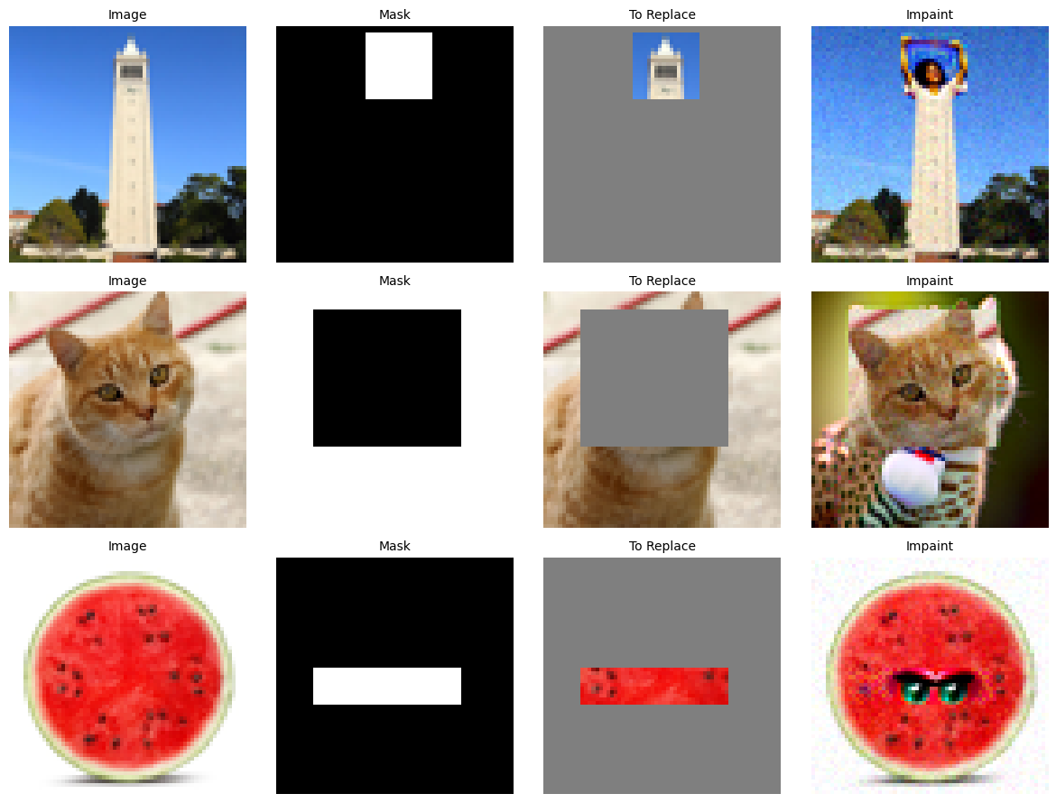
The section implements inpainintg, that is, given an image \( x_{orig} > 1 \), and a binary mask \( m \), we can create a new image that has the same content where
\( m \) is 0, but new content wherever \( m \) is 1:
$$ x_t \leftarrow \textbf{m} x_t + (1 - \textbf{m})
\text{forward}(x_{orig}, t) $$
The test images inpainted are shown below:

1.7.3 Text-Conditional Image-to-image Translation
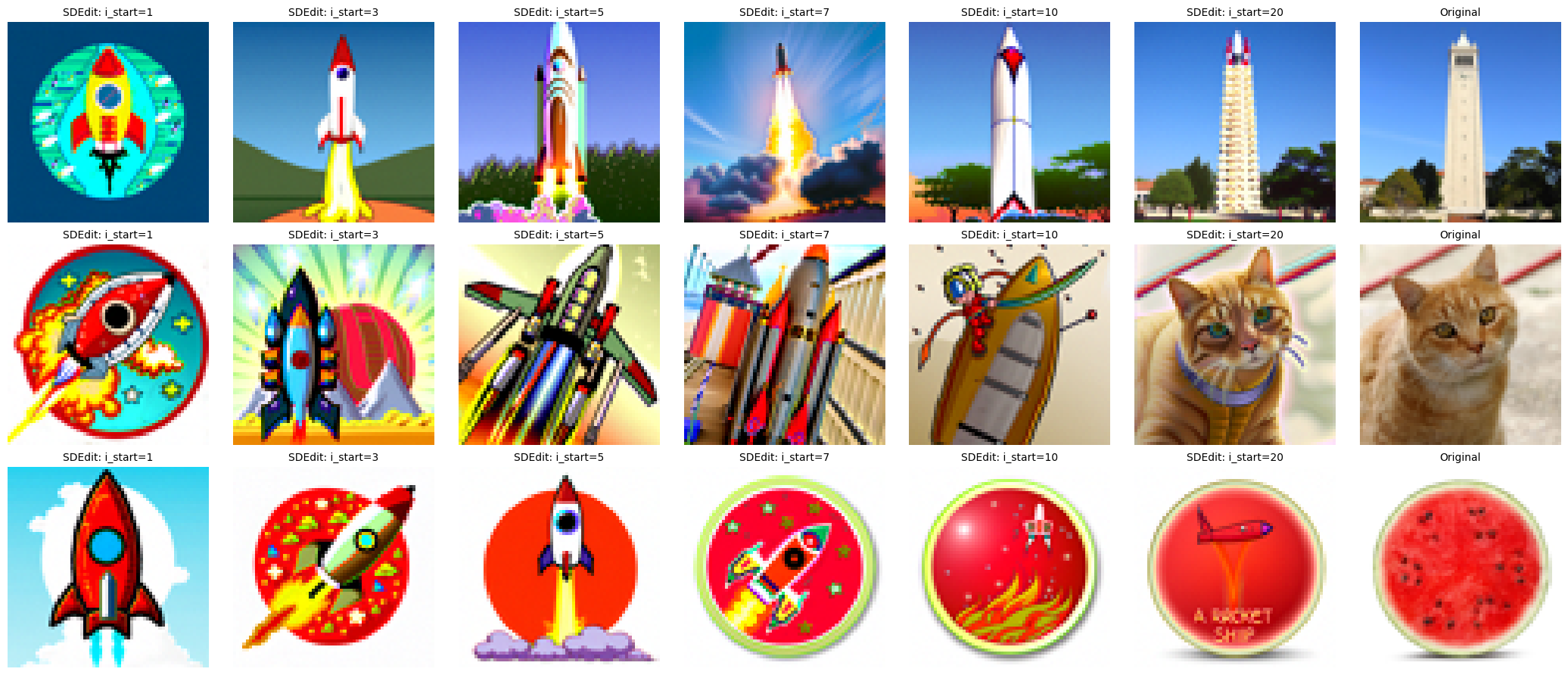
This section applies SDEdit, but guide the projection with a text prompt.
The test images edited at noise levels [1, 3, 5, 7, 10, 20] are shown below:

1.8 Visual Anagrams
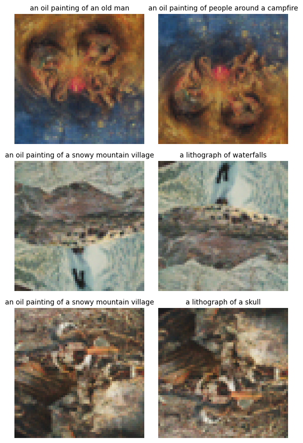
This section implements Visual Anagrams, and create optical illusions with diffusion models.
In this part, it will create an image that looks like one prompt, but when flipped upside down will reveal another prompt.
The image \( x_t \) at step \( t \) is denoised normally with the first prompt, to obtain noise estimate \( \epsilon_1 \),
at the same time flip \( x_t \) and denoise with the second prompt to obtain noise estimate \( \epsilon_2 \) and flip it back.
Then perform a reverse/denoising diffusion step with the averaged noise estimate.
The full algorithm is:
$$ \epsilon_1 = \text{UNet}(x_t, t, p_1) $$
$$ \epsilon_2 = \text{flip}(\text{UNet}(\text{flip}(x_t), t, p_2)) $$
$$ \epsilon = (\epsilon_1 + \epsilon_2) / 2 $$
3 visual anagrams are shown below:

1.9 Hybrid Images
This section implements Factorized Diffusion and create hybrid images.
First create a composite noise estimate, by estimating the noise with two different text prompts,
and then combining low frequencies from one noise estimate with high frequencies of the other. By using a gaussian blur of kernel size 33 and sigma 2, the algorithm is:
$$ \epsilon_1 = \text{UNet}(x_t, t, p_1) $$
$$ \epsilon_2 = \text{UNet}(x_t, t, p_2) $$
$$ \epsilon = f_\text{lowpass}(\epsilon_1) + f_\text{highpass}(\epsilon_2)$$
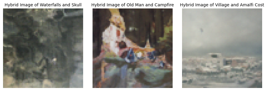
3 hybrid images are shown below:

Part B: Diffusion Models from Scratch
Part 1: Training a Single-Step Denoising UNet
This section builds a simple one-step denoiser.
Given a noisy image
\( z \), we
aim to train a denoiser \( D_\theta \) such that it maps \( z \) to a clean
image \( x \). To do so, we can optimize over an L2 loss:
$$L = \mathbb{E}_{z,x} \|D_{\theta}(z) - x\|^2 $$
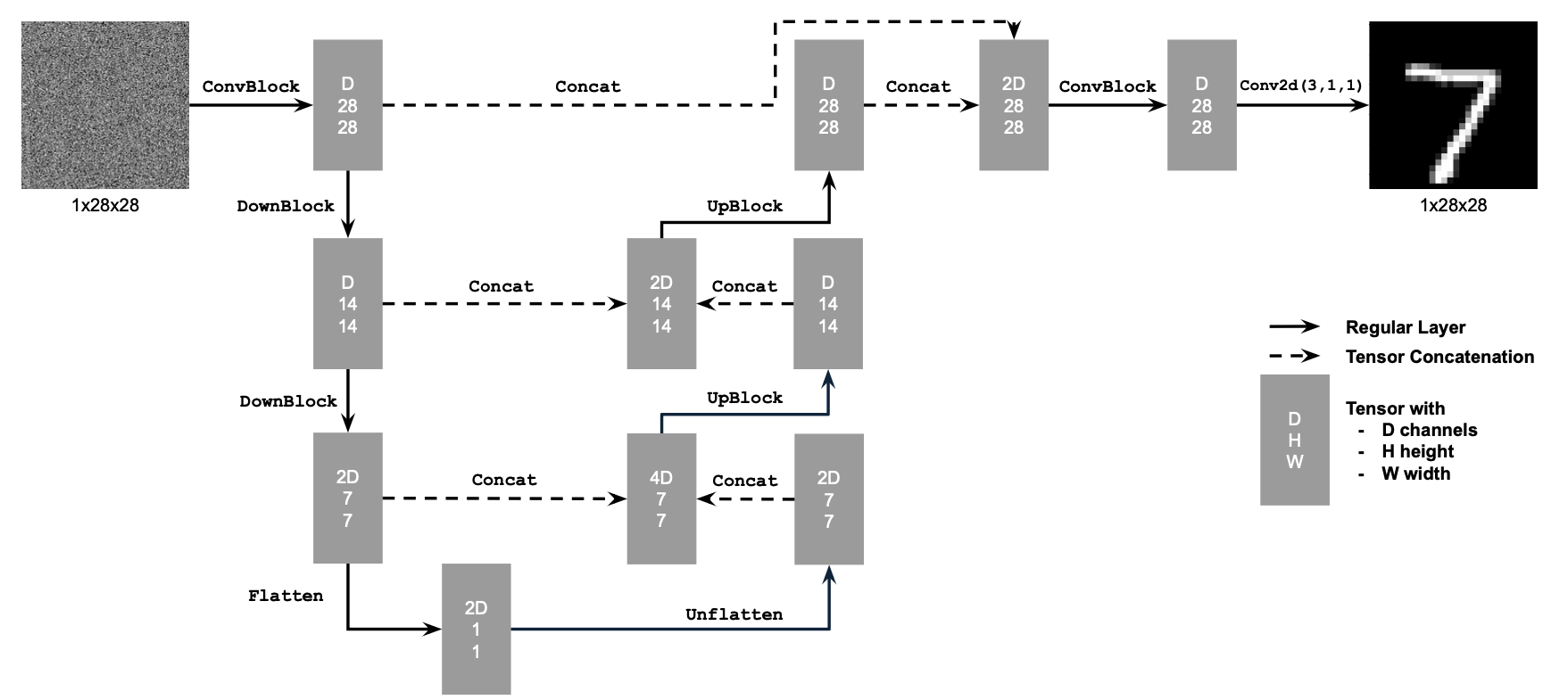
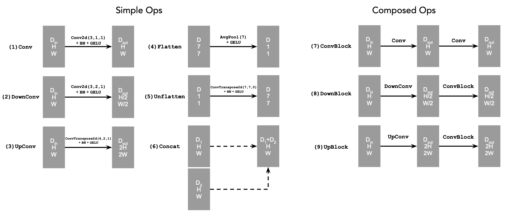
1.1 Implementing the UNet
The implementation follows the diagrams below:


1.2 Using the UNet to Train a Denoiser
To train our denoiser, we need to generate training data pairs of (\( z \), \( x \)), where each
is a clean MNIST digit. For each training batch, we can generate \( z \) from \( x \) using the the following noising process:
$$
z = x + \sigma \epsilon,\quad \text{where }\epsilon \sim N(0, I)
$$
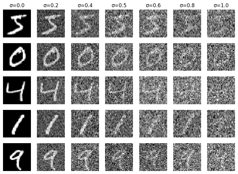
The different noising processes over \(\sigma = [0.0, 0.2, 0.4,
0.5, 0.6, 0.8, 1.0]\), assuming normalized \(x \in [0, 1]\), are shown below:

1.2.1 Training
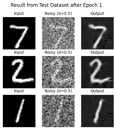
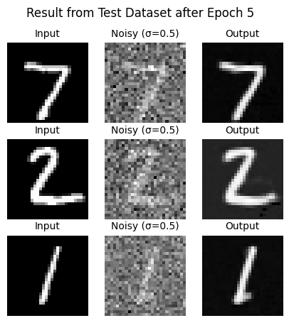
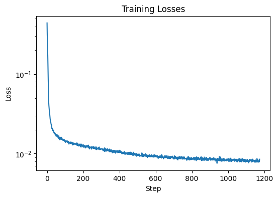
The section trains a denoiser to denoise noisy image \( z \) with \(\sigma = 0.5\) applied to a clean image \( x \),
with dataset torchvision.datasets.MNIST, with batch size 256, for 5 epochs.
The UNet architecture is defined with hidden dimension D = 128. The Adam optimizer is used with learning rate of 1e-4.
The denoised results on the test set after epoch=1 and epoch=5, along with the Training Loss Curve are shown below:


1.2.2 Out-of-Distribution Testing
The denoiser results on test set digits with varying levels of noise \(\sigma = [0.0, 0.2, 0.4,
0.5, 0.6, 0.8, 1.0]\) are shown below:

Part 2: Training a Diffusion Model
This section implements DDPM. The UNet is changed to predict the added noise \( \epsilon \).
The loss function is updated as:
$$L = \mathbb{E}_{\epsilon,x_0,t} \|\epsilon_{\theta}(x_t, t) -
\epsilon\|^2
$$
- Create a list \(\beta\) of length \(T\) such that \(\beta_0 = 0.0001\) and \(\beta_T = 0.02\) and all other elements \(\beta_t\) for \(t \in \{1, \cdots, T-1\}\) are evenly spaced between the two.
- \(\alpha_t = 1 - \beta_t\)
- \(\bar\alpha_t = \prod_{s=1}^t \alpha_s\) is a cumulative product of \(\alpha_s\) for \(s \in \{1, \cdots, t\}\)
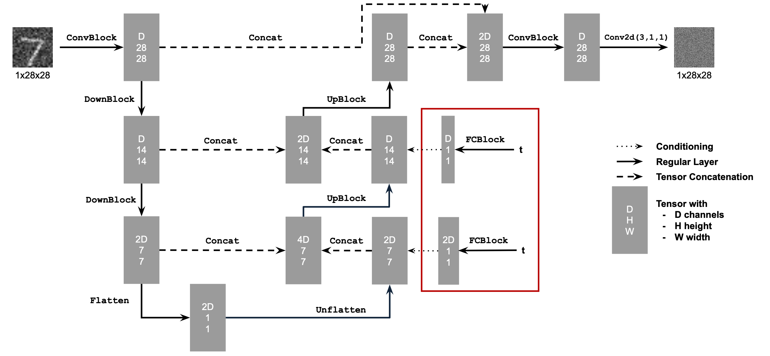
2.1 Adding Time Conditioning to UNet
The conditioned UNet architecture is shown below:


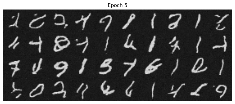
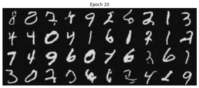
2.2 Training the UNet & 2.3 Sampling from the UNet
To train the time-conditioned model, pick a random image from the training set, a random \(t\)
, and train the denoiser to predict the noise in \(x_t\).
Repeat this for different images and different \( t \) values until the model converges.

The sampling process follows the diagram.

The training loss curve plot, and sampling results for the time-conditioned UNet for 5 and 20 epochs are shown below:


2.4 Adding Class-Conditioning to UNet & 2.5 Sampling from the Class-Conditioned UNet
To make the results better and have more control for image generation, the UNet can be conditioned on the
class of the digit 0-9. This will require adding 2 more FCBlocks to our UNet, for one-hot vector of c, with dropout
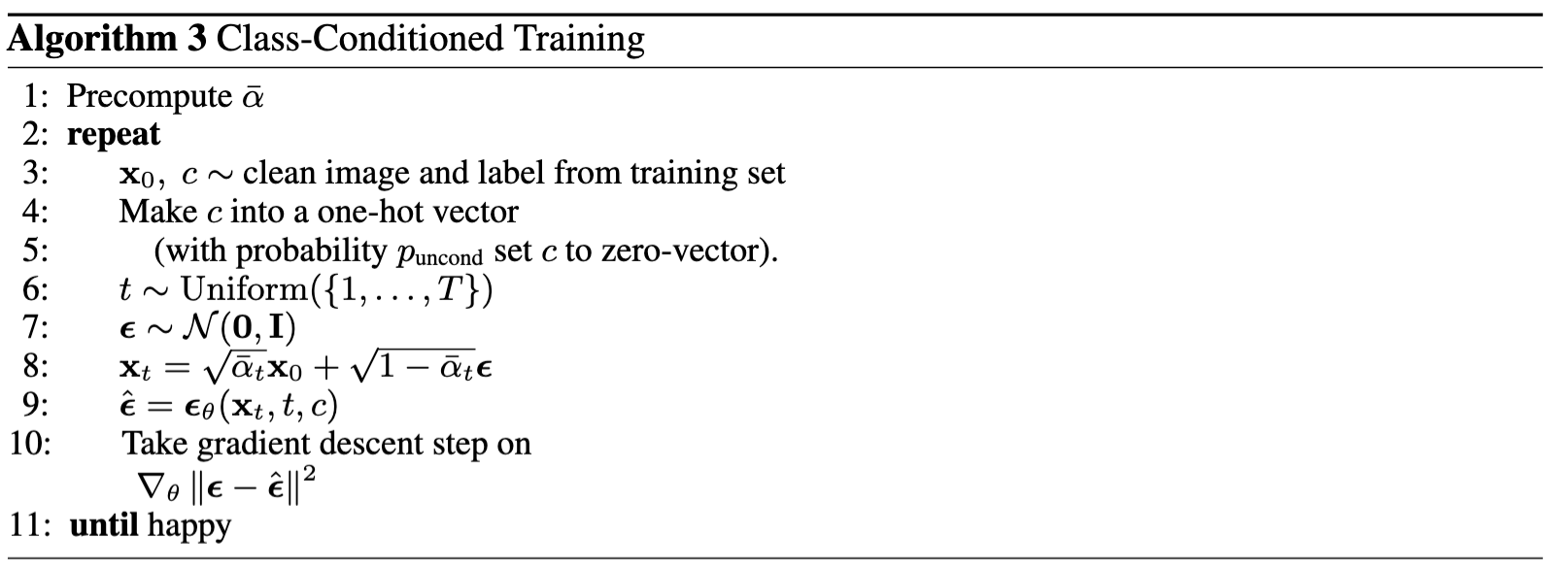
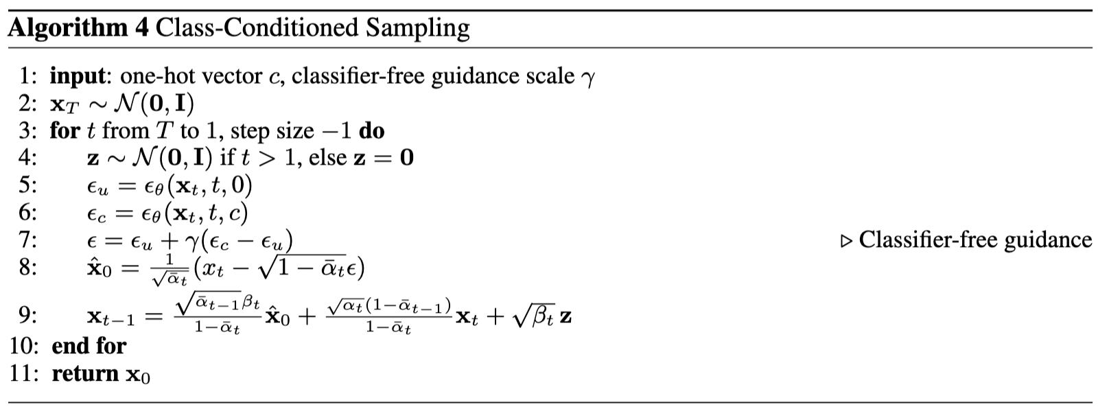
where 10& of the time the class conditioning vector is dropped by setting it to 0. The training and sampling follow the diagrams below:


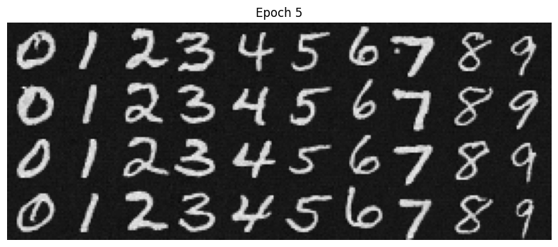
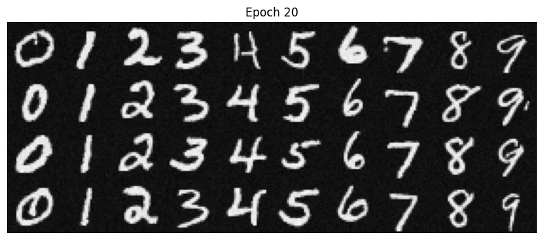
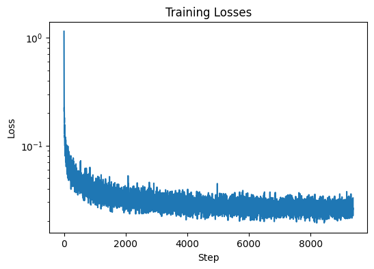
The training loss curve plot, and sampling results for the time-conditioned UNet for 5 and 20 epochs are shown below:
