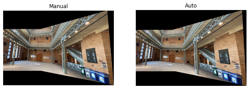
Shoot the Pictures
Acquire the images to be used on the projects by fix the center of projection (COP) and rotate the camera while capturing photos.
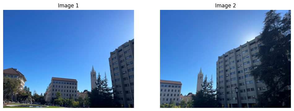
Acquire the images to be used on the projects by fix the center of projection (COP) and rotate the camera while capturing photos.

First, establishing point correspondences by mouse clicking with the tool from project 3.
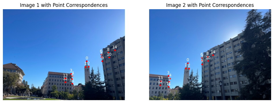
To recover the parameters of the transformation, note that the transformation is a homography: \(Hp=p'\), where H is a 3x3 matrix with 8 degrees:
\[ \begin{bmatrix} a & b & c \\ d & e & f \\ g & h & 1 \end{bmatrix} \begin{bmatrix} x \\ y \\ 1 \end{bmatrix} = \begin{bmatrix} wx' \\ wy' \\ w \end{bmatrix} \]
Expanding the matrix multiplication, the linear systems are:
\[ \begin{bmatrix} x_1 & y_1 & 1 & 0 & 0 & 0 & -x_1'x_1 & -y_1'x_1 \\ 0 & 0 & 0 & x_1 & y_1 & 1 & -x_1'y_1 & -y_1'y_1 \\ x_2 & y_2 & 1 & 0 & 0 & 0 & -x_2'x_2 & -y_2'x_2 \\ 0 & 0 & 0 & x_2 & y_2 & 1 & -x_2'y_2 & -y_2'y_2 \\ &&&&...&&& \end{bmatrix} \begin{bmatrix} a \\ b \\ c \\ d \\ e \\ f \\ g \\ h \end{bmatrix} = \begin{bmatrix} x_1' \\ y_1' \\ x_2' \\ y_2' \\ ... \end{bmatrix} \]
To warp each image towards the reference image with homograph matrix, first, we compute the projected positions of the corners from Image 2 to determine the bounding box of the final warped image. Then, utilizing inverse warping and scipy.interpolate.griddata, we interpolate the pixel values from Image 2 to their new positions in the destination image.
To create image rectification, first marked the position of the four corners on the image, and then define the position of a matched rectangle. Use warpImage to produce the result.
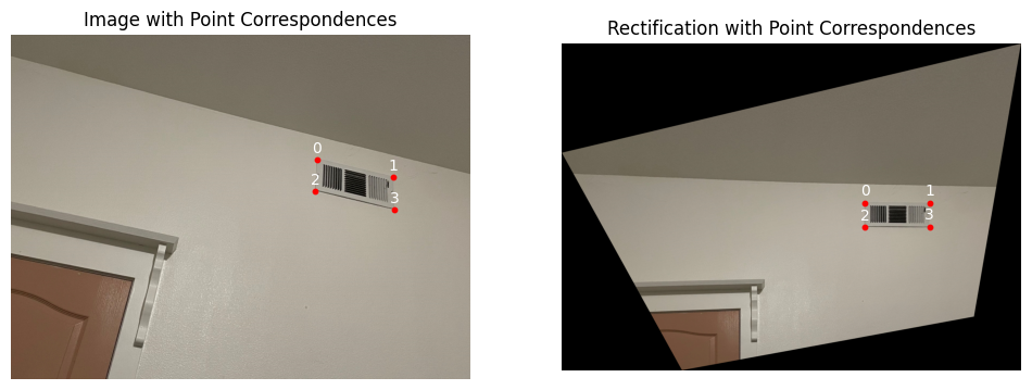
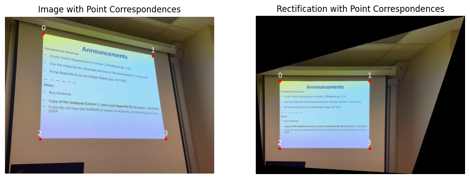
After image warping, the naive overwriting would lead to strong edge artifacts:

To use weight averaging, first compute the distance transform with cv2.distanceTransform, and then compute the weighted linear combination of the two images by using the distance transforms as weights:
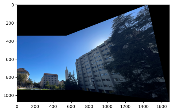
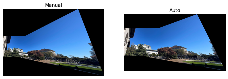
 More results are shown below.


Using sample code harris.py, detect and locate the Harris corner points in a grayscale image.
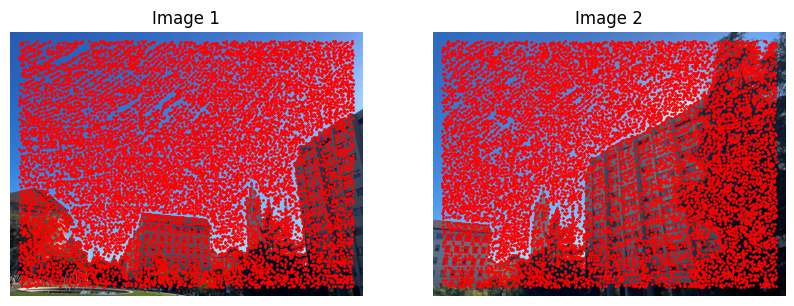
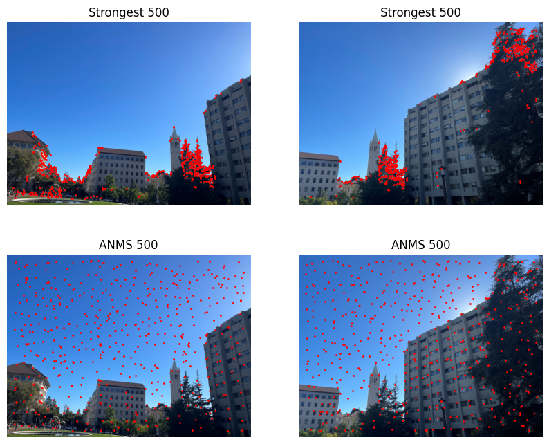
From the MOPS paper, interest points are suppressed based on the corner strength \(f_{HM}\) , and only those that are a maximum in a neighbourhood of radius \(r\) pixels are retained. As the suppression radius decreases from infinity, interest points are added to the list. In practice, the minimum suppression radius \(r_i\) given by\(r_i = min_j |x_i - x_j|, s.t. f(x_i) < c_{robust} f(x_j), x_j \in \mathcal{I}\) is calculated for each corner, then the results of the defined number of interest points are returned from the ordered list.
The two upper images show interest points with the highest corner strength, while the lower two images show interest points selected with adaptive non-maximal suppression with \(c_{robust}=0.9, n_{ip}=500\):
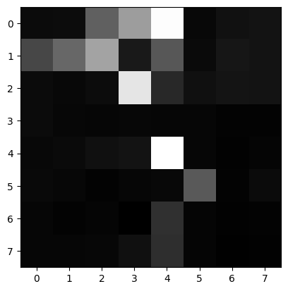
As the paper suggests, a \(8 × 8\) patch of pixels are sampled around the sub-pixel location of the interest point, using a spacing of \(s = 5\) pixels between samples. Then the descriptor vector is normalised so that the mean is 0 and the standard deviation is 1. Here is an example of feature descriptor:
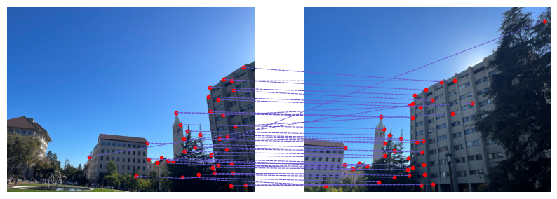
With the use of kd-tree, a ratio threshold of \(e_{1-NN}/e_{2-NN} \) is used to find correct matches by Lowe's technique, based on the assumption that the 1-NN in some image is a potential correct match, whilst the 2-NN in that same image is an incorrect match.
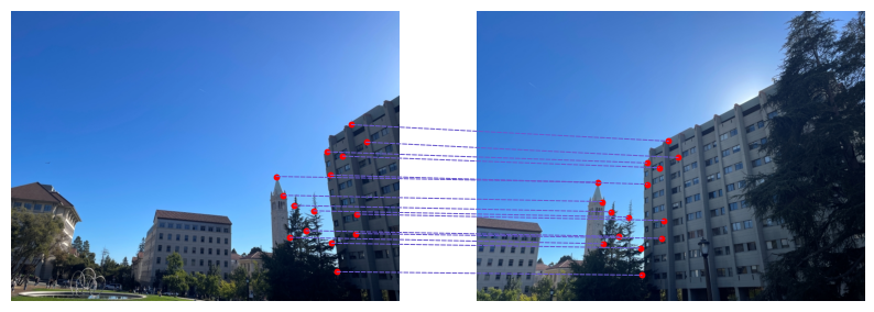
Use 4-point RANSAC as described in class to compute a robust homography estimate and a set of inliers of matches. Within each iteraction, four feature pairs are selected at random, then the exact homography H is computed. The set of inliers is computed where \( \text{dist}(p'_i, H p_i) < \epsilon \). Over the iteractions, the largest set of inliers are kept, and least-squares H estimate on all of the inliers is re-computed.
The final mosaic is presented below, with the warping and blending process same as stated above.
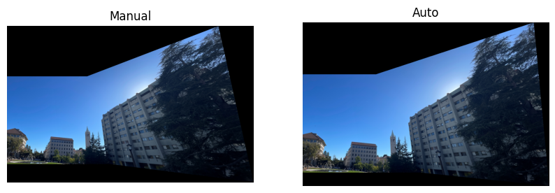
More results are attached below.
